Steps and Instructions
Project setup
This section describes the first steps on the creation of an OBN project, such as the setup of the seismic QGIS project and the initialization of the MantaDesign template. If you have your project already set up and want to read on the actual plugin functionality, you may jump to the next section of the workflow, which begins with the running of ‘1 Generate Seismic Grids’.
1. Create the directories
The first thing you often do when beginning a project is create a folder for it and add two subfolders: ‘ qgis’ and ‘tm’. The first one will be dedicated to the QGIS project and its related files. The second will contain the MantaDesign excel you are going to be working with, and thus you will get here your ‘sardine_outputs’ as well.
ProjectName/
├── qgis/
└── tm/
    └── MantaDesign (xlsm)
Note: This is not a mandatory step, but a good practice done to organize the project, as it may end up with plenty of files and layers.
2. Open and setup MantaDesign
Open your saved MantaDesign.xlsm template. Go to the SARDINE worksheet and create a new Descriptor Sheet with the name of your project. You can do so by tipping the desired name under the grey cell ‘New Descriptor’ and then clicking the New Descriptor button.
On the right-hand side of the SARDINE sheet, you should find a table with the projects and parameters. Write at the top of a blank column the name of the project (Careful! It has to be the exact same name given to the new descriptor sheet). You may now start filling in the ‘source parameters’ and ‘receiver parameters’ of your project in the cells below.
In addition, manually create two new blank worksheets called SL and RL, although not compulsory, these will be helpful in the process of handling data.
Note: Although the chosen name of a project does not concern this manual, it may be interesting to know this: a project name may include 3D if it’s the first time that area has been surveyed. However, if it is not the first time, the name may include 4D, as you are now adding the temporal dimension to the survey (you are shooting in an area you have shot before).
3. Open QGIS and Create a new project
Save it under your new ‘qgis/’ folder.
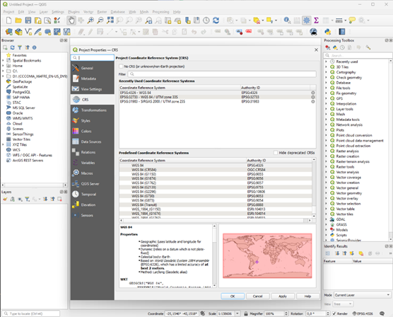
4. Set the correct CRS
The CRS is the Coordinate Reference System. It is necessary to establish the region of the world you are working on, and it is given by the client.

To apply it to your project: Go to the bottom right corner of QGIS → Click to open Project Properties window → Click ’CRS’ on the left menu → Search for and select the given CRS → Click Apply
**5. Upload the source and receiver polygon to QGIS**
The source polygon is the area requested to be shot.
The receiver polygon is the area requested to have nodes deployed on.
They are both usually given by the client in the form of coordinates that mark the vertices.
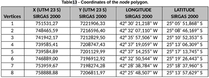

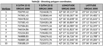
These coordinates are transformed to txt files like these: receiver polygon, source polygon. You can also see the content of the txt files in the Appendix.
Save those txt files under your ‘qgis/’ folder, so:
ProjectName/
├── qgis/
│   ├── Source polygon (txt)
│   └── Receiver polygon (txt)
└── tm/
        └── MantaDesign (xlsm)
We want to have the polygons in our QGIS project. To do so: Go to import layer symbol in the top left corner of QGIS → Open Delimited Text on the left menu → Search for your polygon in the File name → Adjust the dropdowns options to the ones in the slide → Click Add → Repeat for all the polygons
You should now have two polygons showing in your canvas and the two layers showing in your Layer window.
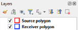

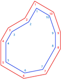
You will get a different style for the uploaded layers. It does not make a difference in the process, but you may change the style by right clicking in the layer → Style → Edit Symbol…
It is a common practice to identify the source as red and the receiver as blue.
Note: You may get additional tables defining more polygons, for example in the case of a densification area. You may upload those to your project with the same logic.
Note: Different clients have different needs; you may not always have polygons among your inputs.
Note: In the Sepia polygon coordinates we have coordinates in both X-Y format and in longitude-latitude format; but the commercial team currently uses only X-Y in their workflow.
1 Generate Seismic Grids
This script creates three temporary layers in your current QGIS project, containing lines and points that define a seismic grid within your polygons’ boundaries.
What the code does is use your input to create the source and receiver grids inside your given source and receiver polygon, respectively. It does so by following the requirements in the boxes below.
1. Open the toolbox
Once your project is set up and the ‘seismicgrids’ plugin is installed, you may proceed to run the Seismic Grids Generator.
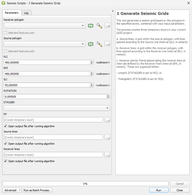
**2. Fill the boxes**
All the necessary inputs at this stage are usually given by the client as a part of the requirements set.
Receiver polygon: choose your receiver polygon layer previously uploaded.
Source polygon: choose your source polygon layer previously uploaded.
RLI: Receiver Line Interval (in meters). It’s the distance between consecutive receiver lines. Also called receiver XL (cross line) distance.
RPI: Receiver Point Interval (in meters). It’s the distance between receiver points (nodes) of the same receiver line. Also called receiver IL (in line) distance.
SLI: Source Line Interval (in meters). It’s the distance between consecutive source lines. Also called source XL (cross line) distance.
AZIMUTH: Azimuth (in degrees). It’s the angle of the source and receiver lines, counting from the top and going clockwise.
Note: QGIS uses by default counterclockwise as positive. This script is adding a ‘-’ in front of the angle to change that logic and having positive be clockwise. That is why in other QGIS’ tools you must add a ‘-’ to refer to the same angle.
QGIS default logic: Generate Seismic Grids logic:
- STAGGER: Type of mesh (YES/NO). It’s the disposition for the receiver points.
YES: hexagonal mesh. Nodes alternated, creating triangles in between lines
NO: rectangular/squared mesh. All the nodes are parallel
3. Run the script
4. Examine the outputs
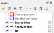
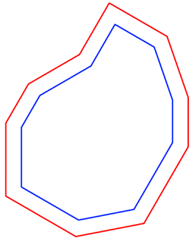
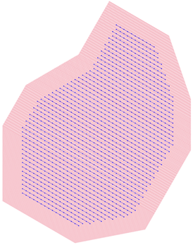
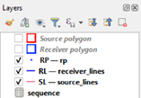
The outputs for this script are three layers that will show both in the Layers menu and in the canvas:
Source lines (SL): A grid of red lines bound inside the source polygon; they are spaced according to the SLI.
Receiver lines (RL): A grid of blue lines bound inside the receiver polygon; they are spaced according to the RLI.
Receiver points (RP): A set of blue points placed along the receiver lines; they are spaced at intervals defined by the RPI and organized following the Type of mesh (STAGGER).
Removed layer Stats (statistics): This layer was removed as the Sequence Generator became a part of the seismic grids plugin, making these parameters no longer needed.
Note: Temporary layers are shown with a symbol next to the name. If QGIS crashes -which tends to happen- these layers will be deleted, so we want to export and save them. This is how: right click on a layer → Export → Save Features As… → save with a name in your ‘qm’ folder. You may also want to copy the style of the temporary layer before deleting it: right click on it → Styles → …. → Finally, delete the temporary layer, as you now have now saved a duplicate.
Note: You can hide layers in QGIS by simply deselecting the check box on the left.
The generated lines are defined by X-Y coordinates that you may find in the Attributes table of each layer. To access this data: select a layer on the Layer menu and find the attribute table symbol either by right clicking the layer or in the upper menu of QGIS. You should now see the attribute table of the selected layer.
Some useful commands are:
Sort the lines by number by clicking on ‘Line’, the first column probably
Select all the values by Ctrl + A and copy them by Ctrl + C
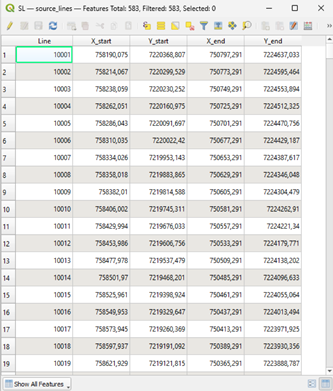
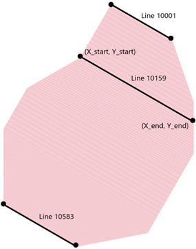
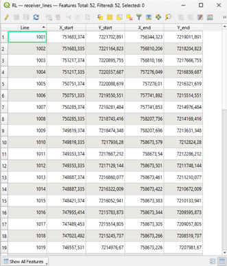
- The Attributes table of the SL and the RL have the following Attributes (Columns):
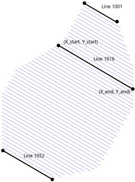
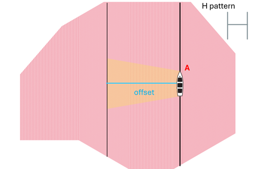
Line (ID): unique number for each source and receiver line. The receiver lines begin with 1001 and continue by adding a unit (1002, 1003…). The amount of source lines is greater, that is why they begin with 10001 and continue from there (10002, 10003…).
X_start and Y_start: X and Y coordinates of the start point of that line.
X_end and Y_end: X and Y coordinates of the end point of that line. That is, you have lines defined by their start and ending point in space
The RP are not relevant for the workflow in QGIS, so we will not go into detail for those.
**5. Copy the data to MantaDesign**
Go to the excel file ‘MantaDesign’. Under the previously created SL and RL sheets, paste all the values in the attribute’s tables of the SL and the RL layer, respectively.
Delete the extra columns so you are left just with: Line, X_start, Y_start, X_end and Y_end.
Source Polygon Irregularity
I think we could and should automatize this calculation. And improve it, it’s quite messy.
If you have a perfect square or rectangular source polygon, the irregularity will be 0. Otherwise, follow the next steps.
Go to QGIS → search for and open the Rotate tool in the Toolbox → select the source lines as the Input layer → in the Rotation box, write the negative value of the azimuth → for the rotation anchor point, click a point near the middle of the polygon (no need to be precise) → click run and wait → you should get a new layer called Rotated
Every time you modify a line (Rotate, Clip, etc) you need to update the coordinates by running this model: ‘Update EOL SOL coords’. Search for and open it in the toolbox → select your modified layer (rotated in this case) → click run → you should get a new layer called Update EOL
Copy the attributes table of the Update EOL layer and paste it in the SL sheet → calculate 1400/SLI → round up and go to that Line ID (e.g.: If 1400/SLI = 29.16, go to line 1030) → if the rotated source lines have a horizontal orientation, calculate abs(X_start1030-X_start1001) and abs(X_end1030-X_end1001); use Y_start and Y_end in case of vertical orientation → drag down formula for the rest of the cells and calculate the average of all the values → that number is considered the source polygon irregularity
Update EOL SOL coords
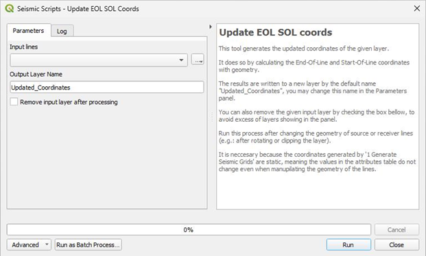
The purpose of this script is to update the End-Of-Line and Start-Of-Line coordinates of QGIS vector layers.
When someone rotates, clips, edits, or reshapes geometries in QGIS, the geometry itself changes, but any attribute fields (like X_start, Y_end, etc.) do not automatically update unless they’re dynamically calculated.
Our source and receiver lines layers have been created using a script, that is why they are static values in the attribute table. Thus, if you rotate or clip one of these line layers the geometry does change (what you visualize on the canvas), but the attribute table does not change, so the X/Y start/end fields are now out of sync. To have them synced again you can run the “Update EOL SOL coords” inside the Seismic Grids plugin.
1. Open the toolbox
**2. Fill the boxes**
No external inputs are needed to run this script.
Input lines: choose the layer containing the lines whose coordinates you want to update (X_start, Y_start, X_end, Y_end).
Output Layer Name: optionally write the name you want the output layer to have.
Remove input layer after processing: check the box to remove the input layer.
3. Run the script 4. Examine the outputs
The output for this script is one permanent layer that will show both in the Layers menu and in the canvas. The lines on the canvas will be the same as the ones given in the input layer; the difference is only in the values of the attribute table.
2 Generate Sequence
This script creates one permanent ‘sequence’ layer in your current QGIS project, containing the sequences for both the source and the receiver’s efforts.
What the code does is use your input to compute the sequence and show it in a new attributes table. It does so by following the requirements in the boxes below.
1. Open the toolbox
You may proceed to run the Sequence Generator once you have a SL layer and a RL layer that combines all the SL and RL of the project, respectively.
If your project consists on just two polygons these layers are just the ones generated by the Seismic Grids Generator but, If you need to consider densified areas or further adjustments, you must previously set up those and combine them, as this process takes just one source lines layer and one receiver lines layer.
**2. Fill the boxes**
Aside from the SL layer and the RL layer, the necessary inputs at this stage are usually given by the client as part of the requirements set.
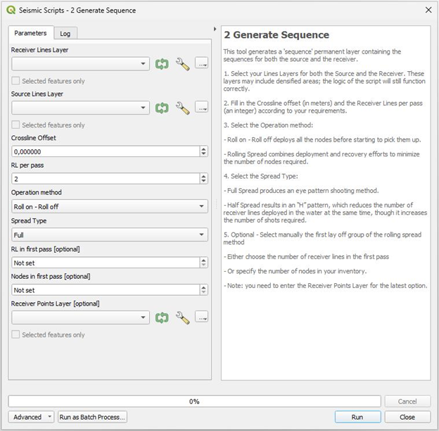
Receiver Lines Layer: choose your receiver lines layer containing all the projects receiver lines that you desire are being considered for the sequence.
Source Lines Layer: choose your source lines layer containing all the projects source lines that you desire are being considered for the sequence.
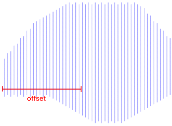
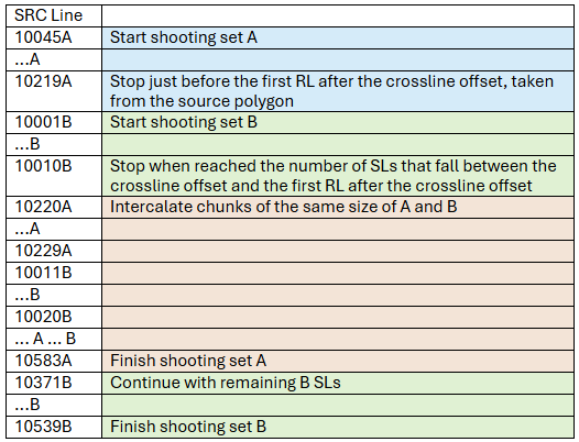
- Crossline offset (in meters). It’s the required minimum distance between the source and receiver efforts.
For the source vessel: minimum distance to the deployment efforts so you can shoot.
For the receiver vessel: minimum distance to the shooting efforts so you can pick up a node. You do not have a crossline offset requirement to being able to deploy nodes, but you are to pick them up.
RL per pass (an integer): It’s the number of RL that are being done at a time. I.e.: it is 2 if you are deploying or recovering two receiver lines in every pass of the receiver vessel. It is usually the number of operating ROVs.
- Operation method: It’s the operation method for the receiver’s efforts; it affects the sorting of the sequence.
Roll on - Roll off: deploys all the nodes before starting to pick them up. You may choose this method if you have as many nodes as required for the project. This is the default method in the toolbox.
Rolling Spread: combines deployment and recovery efforts to minimize the number of nodes required. I.e.: the sorting of the sequence mixes deployment and recovery operations. You may choose this method if you don’t have as many nodes as required for the project.
Static patch: deploys all the nodes, shooting them and after that, recover. As the Roll on - Roll off method, it requires all the nodes.
- Spread Type: It’s the operation method for the source efforts; it affects the length and sorting of the sequence.
<u>Full Spread</u>: produces an “I” pattern shooting method.
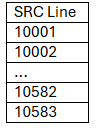
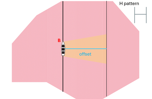
<u>Half Spread</u>: produces an “H” pattern shooting method, which reduces the number of receiver lines deployed in the water at the same time, though it increases the number of shots required.
- Optional: manually choose the chunk that is first deployed in the rolling spread method. You may do so by choosing either the RL or the nodes being first deployed:
<u>RL in first pass</u> [optional] (an integer): It’s the number of RL that you want to first deploy before starting to mix deployment and recovery efforts. It will also be the maximum number of RL in water during the project.
- <u>Nodes in first pass</u> [optional] (an integer): It’s the number of nodes your inventory has. The code calculates the maximum number of RL in water by calculating which line you can completely deploy with the number of nodes available. From then on, it works the same way as the RL in first pass.
Note: for this parameter to work, you need to enter the Receiver Points Layer in the box below, as this layer contains the nodes’ positions.
!! The logic of the sequence and its variability gets a little bit complicated. See more detailed information in the ‘Sequence methods’ section and in the ‘Dependencies’ logic’ section.
3. Run the script
4. Examine the output
The output for this script is one ‘sequence’ layer that will show only in the Layers menu, not in the canvas.
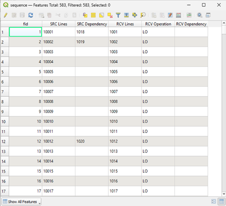
The Attributes table of the sequence has the following Attributes (Columns):
SRC Lines: Line IDs of the SL.
SRC Dependency: Shows the RL that the current SL is dependent on. I.e.: You cannot shoot that SL until the dependent RL has been deployed.
RCV Lines: Line IDs of the RL.
RCV Operation: Shows the operation that corresponds to that RL at that time of the sequence. It can be LO (lay off) or PU (pick up). No dependency will show ever for a LO, only for PUs.
RCV Dependency: Shows the SL that the current RL is dependent on. I.e.: You cannot pick up that RL until the dependent SL has been shot.
5. Copy the data to MantaDesign
Go to the ‘MantaDesign’ excel and paste the sequence in a new sheet, this will give you the ability to make some changes in the sequence, such as the line’s names, the sequence order, the dependencies… Working in a different sheet helps reducing mistakes and also keep a trace of different versions if we need it. Nonetheless, the final sequence shall be pasted in the right columns of your project’s Descriptor sheet, under ‘SRC sequence’ (columns O-P) and ‘RCV sequence’ (columns R-T).
Note that there are two extra columns in the sequences: the Extra hours for the source and the receiver. These are calculated and added manually in later steps of the sardine workflow.
If not done before, you may now also paste the coordinates of your SL and RL to the descriptor sheet of your project, in the right columns under ‘Source lines’ (columns A-E) and ‘Receiver lines’ (columns G-K).
Note: With this workflow it may not be clear why to have these columns first pasted under SL and RL instead of directly in the descriptor sheet. Here it might not be necessary, but it is for more complex projects.
Sequence methods
The sorting of the sequence varies depending on the chosen method for the source and the receiver.
Receiver: Roll on - Roll off method
This method deploys all the nodes in order and then picks them all up in order. That way, what you get in the receiver sequence is something like:
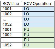
Where 1052 is the last receiver line.
Reminder: the amount of receiver lines recovered or deployed per pass of the receiver vessel is set by the parameter ‘RL per pass’.
Receiver: Rolling Spread method
This method combines deployment and recovery efforts to minimize the number of nodes required. I.e.: the sorting of the sequence mixes deployment and recovery operations.
First, the sequence shows some lines being deployed. The number of lines initially deployed is going to be the maximum number of RL in the water, and by default it’s calculated by a function inside the script (name of the function: _get_max_rl_in_water):
If Full Spread: max_rl_in_water = RL_in_offset * 2 + rl_per_pass + (rl_per_pass - 1)
If Half Spread: max_rl_in_water = RL_in_offset * 1 + rl_per_pass + (rl_per_pass - 1)
Where RL_in_offset is the number of RLs that fall inside the crossline offset distance
Note that, in the calculation of max_rl_in_water, RL_in_offset is multiplied by 2 in the Full Spread and by 1 (stays the same) in the Half Spread.
Note: I do not know why the **max_rl_in_water* is calculated this way. This is how it was done (or better, tried to be done) in the old sequence generator.*
This _get_max_rl_in_water function is used by default to calculate max_rl_in_water, but you may also manually choose that parameter using the ‘RL in first pass’ or the ‘Nodes in first pass’ input options.
Once the sequence deploys the maximum number of RL in water calculated, it starts picking up the first receiver line and then intercalating deployment and recovery passes. Reminder: the amount of receiver lines recovered or deployed per pass of the receiver vessel is set by the parameter ‘RL per pass’.
So, if RL per pass = 2, you will get: …, PU, PU, LO, LO, PU, PU, LO, LO, … As long as there are lines left to be deployed.
Same way, if RL per pass = 3, you get: …, PU, PU, PU, LO, LO, LO, PU, PU, PU, LO, LO, LO, … As long as there are lines left to be deployed.
This way, you never have more RL in water than the calculated max_rl_in_water.
Finally, once the last RL has been deployed, only some RLs remain to be picked up.
Note: in future versions of the ‘seismic grids’ plugin, we could benefit from having different RL per pass for deployment and recovery, which would change the way the sequence is presented.
The final receiver sequence will look something like:
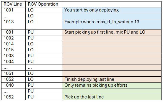
Where 1052 is the last receiver line and RL per pass = 2.
Note that the receiver sequence will always have double the length of the number of RL, as it contains each RL two times: being deployed (LO) and being recovered (PU).
Receiver: Static Patch method
The sequence looks like the Roll on - Roll off method; the only change is in the dependencies. The source lines will have just one dependency on the first line, which corresponds to the last RL (e.g. 10001 -> 1052). The first receiver line in the PU has the dependency of the last SL (e.g 1001 PU ->10060, assuming 10060 is the last SL).
Source: Full Spread method
This method is also usually called ‘I pattern’. It is the most used as it is simpler yet more efficient and only requires one source vessel.
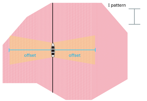
The sequence simply goes through all the SL in order, so:
Where 10583 is the last source line.
By ‘order’ in mean the order of the input. If your Source Lines layer is missing SLs or has extra ones, that will also reflect on the sequence.
Source: Half Spread method
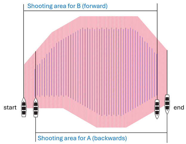
This method is also usually called ‘H pattern’. It is less used as it is more complicated and requires two source vessels or two passes of the same one, we call these A and B. This pattern is chosen when there is a need to reduce the number of nodes deployed in the water at the same time, though it increases the number of shots required.
Each pass of the vessel through the project -A and B- is shot in a different direction, allowing to only have the crossline distance requirement in the direction of the shot, instead of in both directions, as the Full Spread does.
The number of shots is going to be almost doubled in this method, but not exactly:
Therefore, we have two sets of source line IDs (for the Sepia example):
10001B, 10002B, …, 10539B
10045A, 10046A, …, 10583A
Where the original set was from 10001 to 10583.
Now, how are they sorted? Because the source sequence is still only one sequence, not two. Let’s see the logic of it:
First, the sequence shows some ‘A’ SLs: from the beginning to just before the first RL after the crossline offset, taken from the source polygon.
Second, the sequence includes a certain number of ‘B’ SLs starting from the beginning. This number is the same as the number of SLs that fall between the crossline offset and the first RL after the crossline offset (could be 0).
Next, the sequence intercalates chunks of ‘A’ and ‘B’ SLs. These pairs of chunks are the same size, given by the number of SLs that fall between two consecutive RLs. This way, the sequence goes through the ‘A’ SLs adding each time all the SLs between the current and next receiver line; then, it adds the same number of SL for the ‘B’, regardless “where” the ‘B’ set is currently at.
The sequence continues intercalating until the ‘A’ set is finished. Even when all the ‘A’ SLs that fall between RLs have been included, the sequence continues intercalating using the size of the first intercalated chunk.
Finally, when the ‘A’ set has been finished, the remaining ‘B’ SLs are included in the sequence in order.
The final source sequence will look something like:
Dependencies’ logic
The dependencies of the source and receiver lines are always described as:
Dependency for the source: Shows the RL that has to be deployed before you can shoot that SL.
Dependency for the receiver: Shows the SL that has to be shot before you can pick up that RL.
The logic does not change with the receiver method (Roll on - Roll off / Rolling spread) but it does change with the source method (Full or Half Spread), let’s see how:
Full Spread
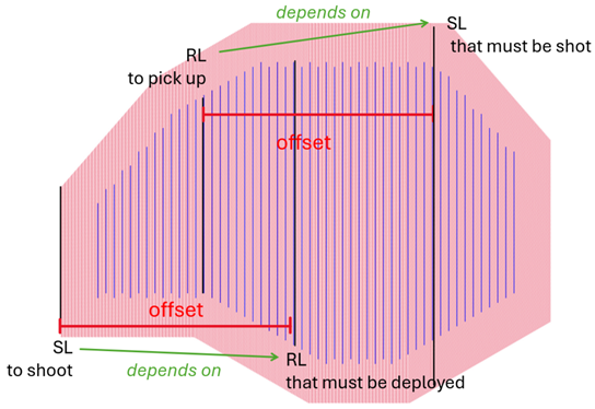
SRC dependency: first RL after the crossline offset distance from the current SL.
RCV dependency: first SL after the crossline offset distance from the current RL.
Half Spread
SRC dependency: closest RL from the left (before) the current SL.
RCV dependency: closest SL from the left (before) the current RL.
Note that, on the half spread, the source dependencies only appear for the ‘A’ set, because the ‘B’ set comes later it has no further dependencies, as long as the sequence is followed. For the same reason, the receiver dependencies of the half spread are from the set ‘B’, as it is the second shooting pass and therefore the RL cannot be picked up before ‘B’ passes.
RL per pass
The number of RL per pass does not change the logic of the dependencies, but it does change how the dependencies are displayed in the sequence.
If RL per pass = 1, then the RLs show their calculated SL dependencies.
However, if RL per pass > 1, then the RLs are meant to be deployed and recovered in groups or chunks. These groups show only one dependency; it appears at the top of the chunk, but is the dependency computed for the last of the chunk. This is because, if you want to pick up 10 RLs together, you need to know when it is okey to pick up the last of the 10.
The final receiver dependencies will look something like:
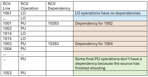
For a Rolling Spread method with Full Spread. Not that in the Roll on - Roll off method the PU operations can also be grouped in chunks, even if they are not intercalated with LO operations.
Extra hours
The extra hours are added once the sequence is set up.
- Add extra hours to the receiver
You may or may not have some or all of the following scenarios that add extra time to the receiver process: Obstructions, Slopes, PIES and Densification. These are explained in detail later in the document.
- Add extra hours to the source
You may or may not have some or all of the following scenarios that add extra time to the source process: Orthogonal lines and Densification. These are explained in detail later in the document.
Obstructions
Obstructions are irregularities on the sea floor (rocks, wreckage…). These irregularities slow down the deployment of the nodes, so they only add extra time to the receiver, not the source (the vessel is not affected by the sea floor). They are represented as points on the map and given by the client.
[add picture]
To calculate how much time the obstructions slow you, we use bathymetry data uploading it to QGIS (could be either given by the client or open source). Then, open ‘Buffer’ in the toolbox → select the point of obstruction → in ‘distance’, write the water depth (bathymetry gives it) → in the other box write 100 → click run → a circle should have been generated around the obstruction → the receiver lines that cross that circle are the ones affected by the obstruction → go to those lines in the descriptor sheet and manually add extra hours in the corresponding cell for the receiver extra time.
The number of hours written in these cells is an estimation linked to the type of obstruction, so it changes mainly depending on the type of obstruction; it’s agreed with operations.
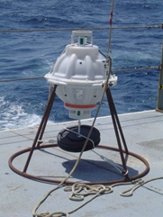
Pies
A PIES, or Pressure Inverted Echo Sounder, is a device sometimes required to be deployed on specific lines, while deploying the nodes. Usually is given by the client in the scope of work. Each time you must deploy or recover one, it adds a few extra hours to the deployment and recovery time. It is manually added in the column of receiver extra hours, and the time may vary between projects, but it stays the same within a project. This extra time is agreed with the operations team.
PIES and OBSTRUCTIONS add time to the extra hours. In the timeline plot they are shown in black, because it is time in where we are ‘not productive’
Slopes
Slopes affect the deployment and recovery of nodes; we usually consider slopes >12°.
General steps to calculate the extra time of a slope: we define the area where the slopes are higher than 12° (or we may already have these areas defined) and then we create polygons in QGIS to delimitate these areas. After that, we clip the receiver lines to these polygons (do not forget to run EOL as well). We continue by taking the distance of these RL clipped and we add the distance in the column ‘slope distance’ in the descriptor worksheet.
Note: Daniela offered to showcase the process in more detail.
[add picture]
Densification – Receiver
There are two types of densifications: in line and cross line.
In the same project, you may have multiple polygons with a different amount of receiver lines per area, leading to what are called sparce areas (high RLI) and dense areas (low RLI). This is called ‘cross line’ densification.
‘Cross line’ densification is the most difficult case. You need to modify the attributes table in QGIS and then work a lot in the excel. This process is shown in the ‘example densification.mp4’ video, write it here!
Instead of different RLIs, you may have receiver lines with a different amount of receiver points, that is, lines with higher RPI and lines with lower RPI. This is called ‘in line’ densification.
‘In line’ densification is the simple case. When required, you only need to do some modifications in the excel, nothing in QGIS.
Note: They would like to have automatization on some or all of this process, as it is the one that takes them the most amount of time. Plus, it is quite easy to make small mistakes in a process this long and manual. Ther mistakes are mainly linked to the need of changing the sequence to match the specific needs of the project.
‘example densification.mp4’
Upload three polygons to QGIS: source, receiver and densification
Run seismic grids with the RPI of the dense area
Open the attributes table of the receiver lines, click on the formula icon and write the appropriate formula, click select. This formula depends on the difference in RLI between dense and sparce area. In the case of RLI = half sparce RLI, then the formula would be (Line-1)%2. A lot of times we need to find a new formula or draw RL by hand. Same goes for SLI.
You should see now each other line selected in the table, search for ‘Clip’ in the Processing toolbox, open it, select Receiver lines as Input layer and densification as Overlay layer, mark the Selected features only on the Input layers (so it selects each other receiver line). Click Run and Close. You should have a Clipped layer now.
Open again the attributes table of the receiver lines layer, click and then to delete.
Search for ‘Merge vector layers’ in the Processing toolbox. As Input, select Clipped and Receiver lines, click OK and Run. You should have a Merged layer now.
Search for ‘Update EOL SOL coords’ in the Processing toolbox. As Input, select Merged layer. Click Run and Close. You should have a With EOL SOL layer now.
Export and save the layers Source lines, Receiver lines, receiver points, Statistics and with eol sol.
Delete all the temporary layers: Source lines, Receiver lines, receiver points, Statistics, with eol sol, merged and clipped.
Open excel, add correct parameters in SARDINE sheet (RPI and RLI of the sparce area I think)
Although the source lines pasted from QGIS to the excel SL sheet are the same, for the receiver lines you get the ones in the with eol sol layer and paste them on the RL sheet.
Now they change the names (Line ID values) of some RL (or SL) because we need to adjust the order. We usually add an A to dense lines (easier to recognize them). We do this process by “hand” (with formulas in excel) but it is different every time we have densification and gets more complicated if we have more densification areas.
Follow the steps under ‘Calculate the source polygon irregularity’
Follow the steps under ‘Run the Sequence Generator’
Follow the steps under ‘Move info to the Descriptor sheet’ but, instead of pasting the sequence in the descriptor, paste it in the RL sheet. Then they move some cells of the edited Line ID column in RL sheet They do an XLOOKUP formula: From the sequence generator we don’t have the correct ID for the lines, so we first reorder the lines, give them the correct number and then we do XLOOKUP for keeping the original dependency.
Then there are a lot of minutes of the video where I am not even sure they are doing something, moving around stuff or just copy-pasting…
In the Descriptor sheet, go to Dist. dense column and write an XLOOKUP formula
Then they do only some small stuffs, but check, because I am lost…
Note: Daniela offered to showcase the process in more detail.
Densification – Source
In the same project, you may have multiple polygons with a different amount of source lines per area, leading to what are called sparce areas (high SLI) and dense areas (low SLI).
[add picture]
The dense area is shot normally but, when you arrive to the border of the dense polygon, frontier with the sparce polygon, the vessels are still going to travel though the dense lines, although not shooting, as they are not required. That is where the extra hours come from: densification adds extra time as the source vessel travels through dense lines in the sparce area.
To add the number of extra hours, they calculate the average extra distance of the polygon and divide it by the source vessel speed (so not very precise). Then, they add it to the correct source lines, which will be all those in which the vessel travels from the dense to the sparce polygon and vice versa. If they notice that the extra distance the vessel must navigate is very different from one part to the other of the polygon, they calculate it more precisely.
Orthogonal lines
These are lines required to be shot by the client, and they are called this way because they are orthogonal to the grid. The time when they are shot also depends on the requirements, so you manually add the decided number of extra hours on the descriptor (check orthogonal lines column).
[add picture]
Apparently, it is not interesting for now to try and automatize this process, it does not take too long and varies a lot from project to project. You add the extra time in the line where you stop the source process to start shooting the orthogonal line, but that always changes so it is complicated.
Run Sardine
Once all the previous steps are finished and you want to run the Sardine code, simply go back to the ‘SARDINE’ sheet in MantaDesign and click the Run Sardine cell, following the directions explained in previous sections.
As the process starts running, a terminal should pop up and you should get some printings on it. When the running is finished, you will get a folder called ‘sardine_outputs’, placed in the same directory as your MantaDesign excel file.
This is the last step of the workflow.

Requirements
ID |
Title |
Status |
|---|---|---|
Descriptor sheet names must match project names exactly. |
open |
|
At least one source and one receiver vessel must be defined. |
open |
|
Source and receiver lines must be defined by start and end coordinates. |
open |